Backpropagation

This is the “engine” of learning. We just calculated the Loss ($L$). Now we need to know: “How much did each weight contribute to this error?”

If we know that increasing weight $w_{11}$ by a tiny bit increases the error, then we should decrease $w_{11}$. This “sensitivity” is called a Gradient.

We calculate these gradients using the Chain Rule of calculus, propagating the error backward from the output to the input.

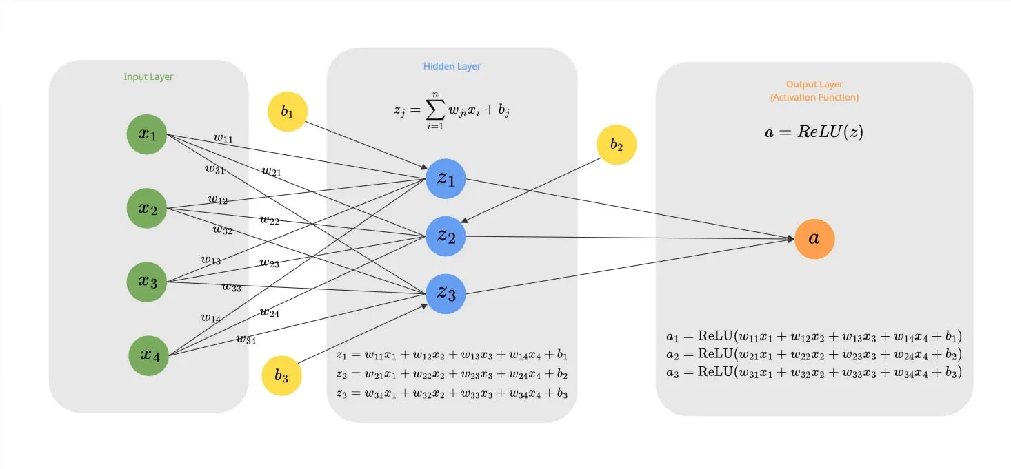
Let’s look at the simple network example that we saw above:

First, let’s calculate the loss function for the output $a$:

(Note: In this specific example, we set the Target to 0 to simplify the math. We want the neuron to learn to output 0.)

To find the gradient of the Loss with respect to a specific weight (e.g., $w_{11}$ connecting Input 1 to Neuron 1), we use the chain rule. We trace the path from the Loss back to the weight:

Path: Loss $\rightarrow$ ReLU $\rightarrow$ Sum $\rightarrow$ Mul $\rightarrow$ $w_{11}$

Using the values from our actual code execution (where $x_1=1.0$, $z \approx 0.964$, $a \approx 0.964$):

1. $\frac{\partial \text{Loss}}{\partial \text{ReLU}}$: The derivative of Mean Squared Error ($\frac{1}{n}\sum(a-y)^2$) with respect to $a$. Since we have $n=3$ neurons:
   • Formula: $\frac{2}{3}(a - \text{Target})$
   • Result: $\frac{2}{3}(0.964 - 0) \approx 0.642$
2. $\frac{\partial \text{ReLU}}{\partial \text{sum}}$: Since $z (0.964) > 0$, the slope is $1$.
3. $\frac{\partial \text{sum}}{\partial \text{mul}}$: $1$.
4. $\frac{\partial \text{mul}}{\partial w_{11}}$: Input $x_1 = 1.0$.

Final Gradient for $w_{11}$:

This positive gradient tells us that increasing $w_{11}$ will increase the error, so we should decrease it.